Approach

As long as the below two conditions hold, we can use Dynamic Programming to solve a problem:

Sub-problem: We can formulate the solution to the original problem as a function of the solutions to “smaller” versions or sub-problems. The “smallest” sub-problems are trivially solved.
Order: A DAG (explicit or implicit) exists such that:
- Node: One node represents one sub-problem.
- Edge: There is an edge from $\texttt{node}_j$ to $\texttt{node}_i$ if computing solution to the $\texttt{subproblem}_i$ requires that the solution to the $\texttt{subproblem}_j$ is already available.
- Must process the nodes in a topologically sorted order.

Given such a DAG, the overall approach is as follows:

def solve(DAG):
    solutions = [] 
    solve_trivial_subproblems(solutions)

    sorted_nodes = topologically_sort(DAG)
    for node_i in sorted_nodes:
        solutions[node_i] = func1( { solution[node_j]: There is an edge from node_j to node_i } )
    
    # Original problem's solution appears in solutions
    return func2(solutions)

Observations

We do not need to perform the topological sorting explicitly. If the inputs to the original problem allow computations to be organized such that we end up processing nodes (or sub-problems) in topologically sorted order, that suffices.
By processing each node (or sub-problem) in topologically sorted order, we can be sure that the solutions to the sub-problems that are required for the current node to be solved, are all available. As a result, for overlapping sub-problems, memoization helps.
func1 is recursive. Going top-down is simpler because the topological order is inferred from func1 on a need-to-know basis. For bottom-up, we need to know the topological order for the entire DAG beforehand.
The total complexity is at least as large as the number of nodes. However, the complexity could actually be dictated by the total number of edges. Because, the total number of edges determines the cost of evaluating func1, the body of the loop. Given the same number of nodes, a dense DAG is computationally more expensive than a sparse DAG.
For optimization problems, where func1 and func2 are max or min, each solution[node_i] has a unique ancestor solution[node_j]. In other words, there is a path (from left to right) through sorted_nodes that leads up to solution[node_i]. To be able to re-construct this path, we could save each solution[node_i]‘s ancestor.
Even if a directed graph seems to exist among the sub-problems, it may not be immediately clear whether it contains a cycle. Since a directed graph is a DAG if and only if it has a topological ordering, it might be easier to approach the problem from the opposite direction. In other words, if there is an inherent order among the sub-problems, it could indicate the presence of a DAG. Trivially solved problems are at the root of the DAG which may suggest how to process the nodes respecting topological order.

Explicit DAG

Shortest paths

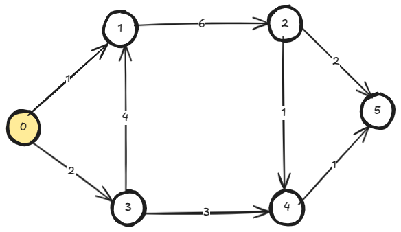
Given a DAG with positive edge weights and a source node, we want to find shortest path distances to every other node from that source node.

In the below DAG, the node 0 is the source.

We can use Dynamic Programming to solve the problem. Because:

Sub-problem: We can formulate the original problem in terms of sub-problems. For example, to be able to reach the node 4, we must either go to node 2 or node 3 first. So, short_dist(4) = min( short_dist(2)+1, short_dist(3)+3 ). The short_dist(0) is trivially solved.
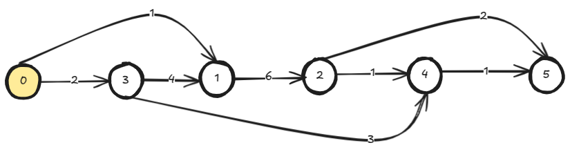
Order: The input itself is a DAG. So, we explicitly do topological sorting and process the nodes in the sorted order.

We do topological sorting first.

from collections import deque

def topo_sort(adj_list: List[List[int]]) -> List[int]:
    n = len(adj_list)
    visited = [False] * n
    topo = deque()
    def dfs(u: int) -> None:
        visited[u] = True
        for v, _ in adj_list[u]:
            if visited[v]:
                continue
            dfs(v)
        topo.appendleft(u)
    for u in range(n):
        if visited[u]:
            continue
        dfs(u)
    return list(topo)

adj_list = [
    [ [1, 1], [3, 2] ],
    [ [2, 6] ],
    [ [4, 1], [5, 2] ],
    [ [1, 4], [4, 3] ],
    [ [5, 1] ],
    []
]
sorted_nodes = topo_sort( adj_list )
print(f"{sorted_nodes=}")
# sorted_nodes=[0, 3, 1, 2, 4, 5]

We solve the nodes or sub-problems in the sorted order. Here func1 is $min(\cdot)$ and func2 is identity.

n = len(adj_list)
dp = [float('inf')] * n
# Solve trivial sub-problem
dp[0] = 0
# Sort topologically
sorted_nodes = topo_sort( adj_list )
for v in sorted_nodes[1:]:
    for u in range(n):
        edges_from_u = adj_list[u]
        for to, w in edges_from_u:
            # Found an edge to current node v
            if to == v:
                dp[v] = min( dp[v], dp[u]+w )

print(f"{dp=}")
# dp=[0, 1, 7, 2, 5, 6]

Since func1 is $min(\cdot)$ , we can save ancestors to be able to re-construct the actual path to a node.

from typing import Optional

def construct_path(current: int, ancestors: List[Optional[int]]) -> List[int]:
    path = deque()
    path.appendleft(current)
    while (prev := ancestors[current]):
        current = prev
        path.appendleft(current)
    path.appendleft(0)
    return list(path)

adj_list = [
    [ [1, 1], [3, 2] ],
    [ [2, 6] ],
    [ [4, 1], [5, 2] ],
    [ [1, 4], [4, 3] ],
    [ [5, 1] ],
    []
]

n = len(adj_list)
dp = [float('inf')] * n
ancestors = [None] * n
# Solve trivial sub-problem
dp[0] = 0
# Sort topologically
sorted_nodes = topo_sort( adj_list )
for v in sorted_nodes[1:]:
    for u in range(n):
        edges_from_u = adj_list[u]
        for to, w in edges_from_u:
            # Found an edge to current node v
            if to == v:
                if (updated_dist := dp[u]+w) < dp[v]:
                    dp[v] = updated_dist
                    ancestors[v] = u

print(f"Shortest distance path to node 5: {construct_path(5, ancestors)}")
# Shortest distance path to node 5: [0, 3, 4, 5]

Implicit DAG

Very first question for a DP problem is: what are the sub-problems? Below example problems are in five categories. All problems in a category define the sub-problem similarly:

Prefix as sub-problem
Pair of prefixes as sub-problem
Knapsack
Subarray as sub-problem
Subtree as sub-problem

Prefix as sub-problem

Input is $a_1, a_2, \ldots, a_n$ and a sub-problem is $a_1, a_2, \ldots, a_i$ .

Number of subproblems: $\mathcal{O}(n)$ .

Longest increasing sub-sequence

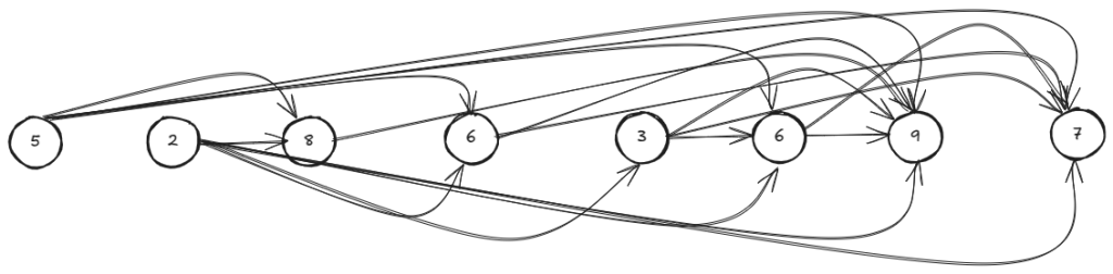
Given a sequence of numbers, we want to find the length of the longest increasing (left-to-right) sub-sequence in it.

For the sequence [5, 2, 8, 6, 3, 6, 9, 7], an increasing sub-sequence is [5, 8] but this is not the longest possible sub-sequence.

We can solve the problem using Dynamic Programming, because:

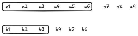
Sub-problem: solutions[ seq[0…i] ] = 1 + max( { solutions[ seq[0…j] ]: j < i } ), solutions[ seq[0…0] ] is trivially solved.
Order: solutions[ seq[0…i] ] does not consider the numbers seq[j] where j > i, so if we process the seq left-to-right, the directed edges will always go towards right and would define a topological order of the sub-problems. Therefore, it is a DAG.

The DAG is like below:

def find_longest_increasing_subsequence(seq: List[int]) -> int:
    n = len(seq)
    
    # Solve trivial sub-problems
    dp = [1] + ([0] * (n-1))

    # Process sub-problems in topologically sorted order
    for i in range(1, n):
        sub_problem_max = 0
        for j in range(i-1, -1, -1):
            # No edge from dp[j] to dp[i]
            # So, dp[j] is not included as a input to func1
            # func1 is max
            if seq[i] <= seq[j]:
                continue
            sub_problem_max = max( sub_problem_max, dp[j] )
        dp[i] = 1 + sub_problem_max

    # func2 is max
    return max(dp)

seq = [ 5, 2, 8, 6, 3, 6, 9, 7 ]
l = find_longest_increasing_subsequence( seq )
print(f"{l=}")
# l=4

Since func1 is $max(\cdot)$ , we can save ancestors to be able to reconstruct the longest increasing sub-sequence.

from typing import Tuple

def find_longest_increasing_subsequence(seq: List[int]) -> Tuple[int, List[int]]:
    n = len(seq)
    
    dp = [1] + ([0] * (n-1))
    prev = [None] * n
    
    for i in range(1, n):
        sub_problem_max = 0
        for j in range(i-1, -1, -1):
            if seq[i] <= seq[j]:
                continue
            if dp[j] > sub_problem_max:
                sub_problem_max = dp[j]
                prev[i] = j
        dp[i] = 1 + sub_problem_max
        
    return dp.index(max(dp)), prev

def construct_subseq(seq: List[int], last_index: int, prev: List[int]) -> List[int]:
    ls = [ seq[last_index] ]
    curr = last_index
    while prev[curr]:
        curr = prev[curr]
        ls.append( seq[curr] )
    ls.reverse()
    return ls

seq = [ 5, 2, 8, 6, 3, 6, 9, 7 ]
last_index, prev = find_longest_increasing_subsequence( seq )
ls = construct_subseq( seq, last_index, prev )
print( f"{ls=}" )
# ls=[2, 3, 6, 9]

Pair of prefixes as sub-problem

Input is $a_1, a_2, \ldots, a_m$ and $b_1, b_2, \ldots, b_n$ . A sub-problem is a pair of prefixes: $a_1, a_2, \ldots, a_i$ and $b_1, b_2, \ldots, b_j$ .

Number of subproblems: $\mathcal{O}(m \cdot n)$ .

Edit distance

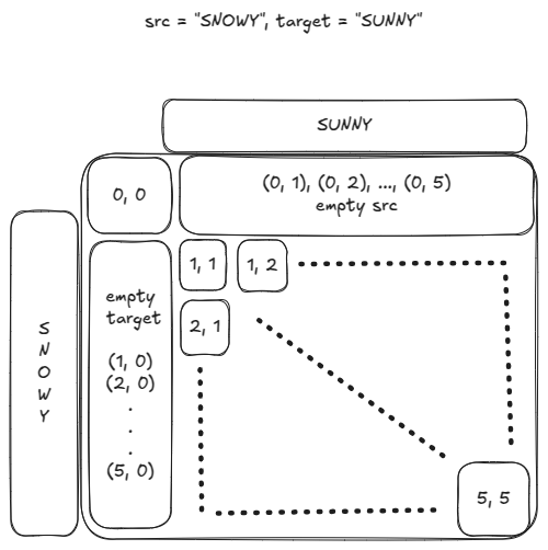
Given a source string and a target string, we want to find the minimum cost to transform source into target. Three operations are allowed:

Delete: We can delete a char from source string
Insert: We can insert a char from target string into source string
Replace: We can replace a char in source with a char in destination

Dynamic Programming can be used because:

Sub-problem: Say we have src[1…m] and target[1…n]. Looking at the last char from both strings, either we can delete src[m], we can insert target[n], or we can replace src[m] with target[n]. So, we define: solutions[ (src[0,1,…i], target[0,1,…j]) ] = min( { 1+solutions[ (src[0,1…i-1], target[0,1…j]) ], 1+solutions[(src[0,1…i], target[0,1…j-1])], delta(i, j)+solutions[(src[0,1…i-1], target[0,1…j-1])] : i <= m and j <= n } ) where diff(i, j) = 0 if src[i]==target[j] else 1. The solution to original problem is solutions[ (src[1…m], target[1…n]) ]. The sub-problems corresponding to empty src string (src[0…0]) or empty target string (target[0…0]) are trivially solved.
Order: The sub-problems can be placed on a (m+1)-by-(n+1) like below. The first row corresponds to the sub-problems: { solutions[ (src[0…0], target[0…j]) ]: j <= n }. Similarly, the first column corresponds to the sub-problems: { solutions[ src[0…i], target[0…0] ]: i <= m }. The DAG’s nodes will be the coordinates of the cells and each node will have exactly three edges from other sub-problems.

The DAG would look like:

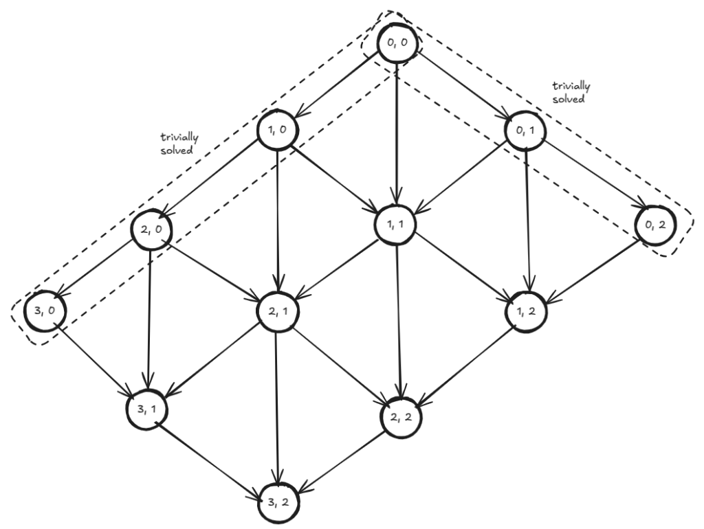
There isn’t a cycle, because all edges go strictly bottom-wards. We have several choices in processing the nodes (or sub-problems) and still maintain topological ordering. We can process each level from top to bottom which would be processing the grid one diagonal at a time. We can process each path going rightwards (grid’s row) or each path going leftwards (grid’s column).

from typing import List, Optional

def construct_ops(dp: List[List[int]], src: str, target: str) -> List[str]:
    ops = []
    i, j = len(dp)-1, len(dp[0])-1
    while i > 0 and j > 0:
        delete_cost  = dp[i-1][j  ] + 1
        insert_cost  = dp[i  ][j-1] + 1
        replace_cost = dp[i-1][j-1] + (0 if src[i-1] == target[j-1] else 1)
        if dp[i][j] == delete_cost:
            ops.append(f"delete {src[i-1]}")
            i -= 1
        elif dp[i][j] == insert_cost:
            ops.append(f"insert {target[j-1]}")
            j -= 1
        else:
            ops.append("no-op" if src[i-1] == target[j-1] else f"replace '{src[i-1]}' with '{target[j-1]}'")
            i -= 1
            j -= 1
    ops.reverse()
    return ops
    

def compute_edit_distance(src: str, target: str) -> Tuple[int, List[str]]:
    m, n = len(src), len(target)
    # src    on y axis or vertical   or rows
    # target on x axis or horizontal or columns
    # 0-th row corresponds to subproblems with empty src
    # 0-th col corresponds to subproblems with empty target
    # i-th row in dp corresponds to (i-1)-th char in src
    # j-th col in dp corresponds to (j-1)-th char in target
    dp = [
        [0 for _ in range(n+1)] for _ in range(m+1)
    ]
    # Solve trivial sub-problems
    # Solve 0-th row, src is empty
    # insert all chars from target into src to match target
    for col in range(1, n+1):
        dp[0][col] = dp[0][col-1] + 1
    # target is empty
    # Solve 0-th col, target is empty
    # delete all chars from src to match target
    for row in range(1, m+1):
        dp[row][0] = dp[row-1][0] + 1

    for row in range(1, m+1):
        for col in range(1, n+1):
            # Sub-problem (row, col) has edges from three sub-problems:
            # 1. (row-1, col  ): delete src char
            # 2. (row,   col-1): insert target char
            # 3. (row-1, col-1): (may be) replace src char
            # func1: min()
            dp[row][col] = min(
                dp[row-1][col  ] + 1,
                dp[row  ][col-1] + 1,
                dp[row-1][col-1] + (0 if src[row-1] == target[col-1] else 1)
            )

    # func2: select last cell
    return dp[m][n], construct_ops(dp, src, target)

src, target = "SNOWY", "SUNNY"
edit_dist, ops = compute_edit_distance( src, target )
print(f"{edit_dist=}, {ops=}")
# edit_dist=3, ops=['no-op', 'insert U', 'no-op', "replace 'O' with 'N'", 'delete W', 'no-op']

Knapsack

Knapsack with repeat

Take items with weight ( $w_i$ ) and value ( $v_i$ ) in a knapsack that can carry a total weight of $W$ with the goal of maximizing the total value in the knapsack. Every item has many copies. So, apart from the constraint on the knapsack’s total weight, there is no limit on how many copies of an item we can take.

Sub-problem

$dp\left[W\right] = \begin{cases} 0, & \text{if } W = 0 \\ \max\left( \left\{ dp[W-w_i]+v_i : w_i \le W \right\} \right), & \text{otherwise} \end{cases}$ .

We take $max(\{\}) = 0$ .

Order

Increasing order of $W$ .

With $n$ items, time: $\mathcal{O}(W)$ , space: $\mathcal{O}(W)$ .

def knapsack_with_repeat(items: List[List[int]], total_weight: int) -> int:
    dp = [0] * (total_weight+1)
    for W in range(1, len(dp)):
        for w, v in items:
            dp[W] = max( dp[W], dp[W-w]+v if w <= W else 0 )
    return dp[total_weight]

items = [
    [6, 30], # [w_i, v_i]
    [3, 14],
    [4, 16],
    [2,  9]
]
total_weight = 10
total_value = knapsack_with_repeat(items, total_weight)
print(f"{total_value=}")
# total_value=48

Knapsack without repeat

Only difference with “Knapsack with repeat” is, we can take an item at most once.

Sub-problem

Trivial sub-problems are when $W = 0$ or the list of items is empty.

$dp[W, i] = \begin{cases} 0, & \text{if } W=0 \\ dp[W, i-1], & \text{if } w_i > W \\ \max\left(dp[W-w_i, i-1]+v_i, dp[W, i-1]\right), & \text{otherwise} \end{cases}$

We take $max(\{\}) = 0$ .

Order

Sub-problems form a grid, row-wise.

With $n$ items, time: $\mathcal{O}(n \cdot W)$ , space: $\mathcal{O}(n \cdot W)$ .

def knapsack_without_repeat(items: List[List[int]], total_weight: int) -> int:
    n = len(items)
    dp = [
        [0]*(total_weight+1) for _ in range(n+1)
    ]
    for i in range(1, n+1):
        w, v = items[i-1]
        for W in range(1, total_weight+1):
            dp[i][W] = max(
                dp[i-1][W-w]+v if w <= W else 0, # take
                dp[i-1][W  ]                     # leave
            )
    return dp[n][total_weight]

items = [
    [6, 30], # [w_i, v_i]
    [3, 14],
    [4, 16],
    [2,  9]
]
total_weight = 10
total_value = knapsack_without_repeat(items, total_weight)
print(f"{total_value=}")
# total_value=46

Subarray as sub-problem

Input is $a_1, a_2, \ldots, a_n$ and a subproblem is $a_i, a_{i+1}, \ldots, a_j$ .

Number of subproblems: $\mathcal{O}(n^2)$ .

Chain matrix multiplication

Given a sequence of $n$ matrices: $\left[ A_1, A_2, A_3, \ldots, A_n \right]$ , we want to find the minimum cost to compute their product: $A_1 \cdot A_2 \cdot A_3 \ldots A_n$ . The cost here is the total count of multiplications. The cost varies depending on how we parenthesize the matrices to carry out the multiplications.

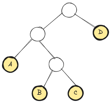
The parenthesized multiplication can be represented as a binary tree. For example $A \cdot \left( \left( B \cdot C \right) \cdot D\right)$ can be thought as:

The number of distinct such trees is the number of distinct parenthesizations of the matrices. Say $B(n)$ is the number of distinct binary trees with $n$ leaves. Then, $B(n) = \sum_{k=1}^{n-1} B(k) \cdot B(n-k)$ . If we compare $B(n)$ ‘s recurrence relation with that of Fibonacci number ( $F(n) = F(n-1) + F(n-2)$ ), we see $B(n) \ge F(n)$ . In other words, there are at least $2^n$ different parenthesizations of a sequence of $n$ matrices; brute force checking of each of these is going to be very inefficient.

Sub-problem

Facts about matrix multiplication

The cost of multiplying matrix $A^{m \times n}$ with the matrix $B^{n \times p}$ is $m \cdot n \cdot p$ . Because the product matrix will have $m \cdot p$ entries and each entry requires a $n$ -sized dot product.
Say we have already found the two products: $A_i^{r_i \times c_i} \cdot A_{i+1}^{r_{i+1} \times c_{i+1}} \ldots A_k^{r_k \times c_k}$ and $A_{k+1}^{r_{k+1} \times c_{k+1}} \cdot A_{k+2}^{r_{k+2} \times c_{k+2}} \ldots A_j^{r_j \times c_j}$ . The cost of multiplying these two products is $r_i \cdot c_k \cdot c_j$ .

Say $C(i, j)$ is the minimum cost for multiplying the sequence of matrices: $A_i, A_{i+1}, \ldots A_{j}$ . Note, $i \le j$ .

$C(i, j) = \begin{cases} 0, & \texttt{if } i=j \\ \min\left( \left\{ C(i, k)+C(k+1, j)+r_i \cdot c_i \cdot c_j : i \le k < j \right\} \right), & \texttt{otherwise} \end{cases}$

The subproblems reside on a two-dimensional grid. Say $i$ is the row index and $j$ is the column index. The solution to the original problem is then $C(0, n-1)$ and it will be on the last grid-cell on the first row. Also, since $i \le j$ , all subproblems reside on or above the main diagonal. So, the subproblems actually form a triangle.

Order

The size of a subproblem is $(j-i)$ , because between $i$ and $j$ , there are $(j-i)$ different values $k$ can take on. The edges always go from smaller sized subproblems to the bigger sized subproblems. For example, a 3-sized sub-problem can have edges from 2-, 1-, 0-sized subproblems but not from 4-, 5-, etc. sized subproblems. Thus, processing the subproblems in increasing order of size gives us a topological ordering.

Time: $\mathcal{O}(n^3)$ , space: $\mathcal{O}(n^2)$ .

def compute_min_mult_cost(matrices: List[List[int]]) -> int:
    n = len(matrices)
    dp = [
        [0]*n for _ in range(n)
    ]
    for sz in range(1, n):
        for i in range(0, n-sz):
            j = i+sz
            sub_min = float('inf')
            for k in range(i, j):
                sub_min = min(
                    sub_min,
                    dp[i][k] + dp[k+1][j] + matrices[i][0]*matrices[k][1]*matrices[j][1]
                )
            dp[i][j] = sub_min
    return dp[0][n-1]

matrices = [
    [50,  20], # A: 50-by-20 matrix
    [20,   1], # B
    [ 1,  10], # C
    [10, 100]  # D
]

cost = compute_min_mult_cost(matrices)
print(f"{cost=}")
# cost=7000

unreasonably effective

Dynamic Programming

Approach

Observations

Explicit DAG

Shortest paths

Implicit DAG

Prefix as sub-problem

Longest increasing sub-sequence

Pair of prefixes as sub-problem

Edit distance

Knapsack

Knapsack with repeat

Sub-problem

Order

Knapsack without repeat

Sub-problem

Order

Subarray as sub-problem

Chain matrix multiplication

Sub-problem

Order

Subtree as sub-problem

Largest independent set of tree

Leave a comment Cancel reply

Dynamic Programming

Approach

Observations

Explicit DAG

Shortest paths

Implicit DAG

Prefix as sub-problem

Longest increasing sub-sequence

Pair of prefixes as sub-problem

Edit distance

Knapsack

Knapsack with repeat

Sub-problem

Order

Knapsack without repeat

Sub-problem

Order

Subarray as sub-problem

Chain matrix multiplication

Sub-problem

Order

Subtree as sub-problem

Largest independent set of tree

Share this:

Leave a comment Cancel reply