Graph Traversal

Say a graph’s vertex set is $V$ and edge set is $E$ . We want to traverse the graph efficiently, therefore, we want to visit each vertex and each edge exactly once.

An edge has two ends: a from and a to. In the edge $(B \rightarrow C)$ we can consider $B$ as from and $C$ as to. The basic traversal strategy is to consider each vertex in the from role exactly once and look at all its to‘s to find not-yet-considered from roles. To avoid putting a vertex in the from role twice, as soon as we decide to consider it in the from role, we mark it as visited.

So, during traversal $V$ is partitioned into two subsets: visited and not-visited:

We can visit the “not-visited” subset in many different orders. Two among these orders enable us to efficiently answer different questions about the graph: DFS and BFS.

DFS

We visit not-visited vertices as we find them and backtrack only when there are no more not-visited to‘s.

DFS can explore a graph in $\mathcal{O}( |V| + |E| )$ time. Piggybacking on the precompute() or postcompute() in DFS, we can solve various problems.

def explore(u, adjacency_list, visited) -> None:
    visited[u] = True
    
    precompute()

    for v in adjacency_list[u]:
        if visited[v]:
            continue
        explore(v, adjacency_list, visited)

    postcompute()

def dfs(adjacency_list: List[List[int]]) -> None:
    n = len(adjacency_list)
    visited = [False] * n
    for u in range(n):
        if visited[u]:
            continue
        explore(v, adjacency_list, visited)

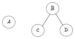
Is undirected graph connected?

Check if all vertices belong to a single connected component.

Time: $\mathcal{O}(|V| + |E|)$ . Space: $\mathcal{O}( |V| + |E| )$ .

def dfs(u: int, adj_list: List[List[int]], visited: List[bool], ccnum: List[int], cc: int) -> None:
    visited[u] = True
    ccnum[u] = cc
    for v in adj_list[u]:
        if visited[v]:
            continue
        dfs(v, adj_list, visited, ccnum, cc)

def find_connected_components(adj_list: List[List[int]]) -> List[int]:
    n = len(adj_list)
    ccnum, cc = [0] * n, 0
    visited = [False] * n
    for u in range(n):
        if visited[u]:
            continue
        dfs(u, adj_list, visited, ccnum, cc)
        cc += 1
    return ccnum

def is_connected_undirected(adj_list: List[List[int]]) -> bool:
    ccnum = find_connected_components(adj_list)
    return len(set(ccnum)) == 1

adj_list = [
    [1, 4],         # 0
    [0],            # 1
    [3, 6, 7],      # 2
    [2, 7],         # 3
    [8, 9],         # 4
    [],             # 5
    [2, 7, 10],     # 6
    [2, 3, 10, 11], # 7
    [4, 9],         # 8
    [4, 8],         # 9
    [6, 7],         # 10
    [7]             # 11
]

connected = is_connected_undirected( adj_list )
print(f"{connected=}")

adj_list2 = [
    [1, 2], # 0
    [0],    # 1
    [0, 3], # 2
    [0, 2]  # 3
]

connected = is_connected_undirected( adj_list2 )
print(f"{connected=}")

# connected=False
# connected=True

Categorize directed edges

A directed edge $(u \rightarrow v)$ can belong to one of four categories based on when $u$ sees $v$ during DFS.

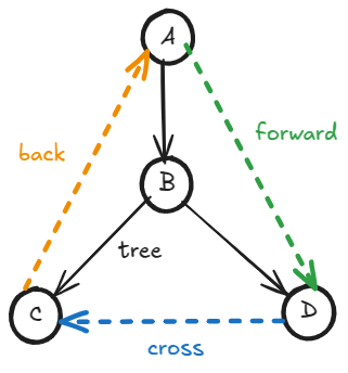
Tree edge: $v$ is a child of $u$ . The vertex $v$ had not been visited when $u$ saw it. If the edge $(u \rightarrow v)$ represents that the task $u$ depends on the task $v$ , then $v$ must be done before we can do $u$ . The vertex $v$ is about to be put in the recursion call stack.
Forward edge: $v$ is a descendant of $u$ . The vertex $v$ had already been entered and exited — therefore completely processed. The vertex $v$ is not in the recursion call stack.
Back edge: $v$ is an ancestor of $u$ . The vertex $v$ had been entered but not exited yet. Therefore, $v$ is still in the call stack.
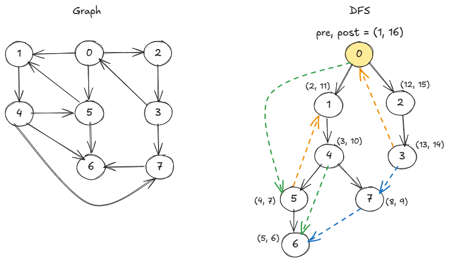
Cross edge: $v$ is neither descendant nor ancestor of $u$ . The vertex $v$ has been entered and exited — therefore completely processed; $v$ is not in the call stack. Additionally, down from their least common ancestor, the subtrees $u$ and $v$ belong to, could have been processed concurrently without breaking dependency constraints.

From DFS pre- and post-times, we can categorize the edges.

def dfs(u, adj_list, visited, clock, pre, post) -> None:
    visited[u] = True
    
    clock[0] += 1
    pre[u] = clock[0]

    for v in adj_list[u]:
        if visited[v]:
            continue
        dfs(v, adj_list, visited, clock, pre, post)

    clock[0] += 1
    post[u] = clock[0]

def compute_pre_post_time(adj_list: List[List[int]]) -> Tuple[List[int], List[int]]:
    n = len(adj_list)
    visited = [False] * n
    pre, post = [0] * n, [0] * n
    clock = [0]

    for u in range(n):
        if visited[u]:
            continue
        dfs(u, adj_list, visited, clock, pre, post)

    return pre, post

def categorize_edges(adj_list: List[List[int]]) -> Dict[str, List[List[int]]]:
    pre, post = compute_pre_post_time( adj_list )
    n = len(adj_list)
    cat = defaultdict(list)
    for u in range(n):
        for v in adj_list[u]:
            edge = [u, v]
            if pre[u] < pre[v] < post[v] < post[u]:
                cat["tree_or_forward"].append( edge )
            elif pre[v] < pre[u] < post[u] < post[v]:
                cat["back"].append( edge )
            else:
                cat["cross"].append( edge )
    return cat

adj_list = [
    [1, 2, 5], # 0
    [4],       # 1
    [3],
    [0, 7],
    [5, 6, 7],
    [1, 6],
    [],
    [6]
]

cat = categorize_edges( adj_list )
print(f"{cat=}")

# cat=defaultdict(<class 'list'>, {'tree_or_forward': [[0, 1], [0, 2], [0, 5], [1, 4], [2, 3], [4, 5], [4, 6], [4, 7], [5, 6]], 'back': [[3, 0], [5, 1]], 'cross': [[3, 7], [7, 6]]})

Is directed graph acyclic?

A directed graph has a cycle if and only if DFS finds a back edge.

During DFS, for an edge $(u \rightarrow v)$ , if $v$ has already been entered but not yet exited and $pre[v] < pre[u]$ , then $(u \rightarrow v)$ is a back edge. Or, if $v$ has already been visited and it is still in the stack ( $post[v] = 0$ ), it is a back edge.

# def is_back_edge(u, v, pre, post) -> bool:
#     # v has not been entered yet
#     if pre[v] == 0:
#         return False
#     # v has already been exited
#     if post[v] != 0:
#         return False
#     # v is not an ancestor
#     if pre[v] > pre[u]:
#         return False
    
#     return True

def is_back_edge(u: int, v: int, visited: List[bool], post: List[int]) -> bool:
    return visited[v] and post[v] == 0

def has_back_edge_dfs(u, adj_list, visited, clock, pre, post) -> bool:
    visited[u] = True

    clock[0] += 1
    pre[u] = clock[0]

    for v in adj_list[u]:
        if is_back_edge(u, v, pre, post):
            return True
        if visited[v]:
            continue
        if has_back_edge_dfs(v, adj_list, visited, clock, pre, post):
            return True
    
    clock[0] += 1
    post[u] = clock[0]

    return False
    
def has_directed_cycle(adj_list: List[List[int]]) -> bool:
    n = len(adj_list)
    visited = [False] * n

    clock = [0]
    pre, post = [0]*n, [0]*n

    for u in range(n):
        if visited[u]:
            continue
        if has_back_edge_dfs(u, adj_list, visited, clock, pre, post):
            return True

    return False

adj_list_with_cycle = [
    [1, 2, 5], # 0
    [4],       # 1
    [3],
    [0, 7],
    [5, 6, 7],
    [1, 6],
    [],
    [6]
]

has_cycle = has_directed_cycle( adj_list_with_cycle )
print(f"{has_cycle=}")

adj_list_without_cycle = [
    [2],
    [0, 3],
    [4, 5],
    [2],
    [],
    []
]

has_cycle = has_directed_cycle( adj_list_without_cycle )
print(f"{has_cycle=}")
# has_cycle=True
# has_cycle=False

Topological sort

By DFS post

For a DAG, vertices in decreasing order of DFS post is a topologically sorted (or linearized) order. If we process the vertices in this order, edges will always flow from earlier to later vertices.

def explore(u: int, adj_list: List[List[int]], visited: List[bool], topo_order: List[int]) -> None:
    visited[u] = True
    for v in adj_list[u]:
        if visited[v]:
            continue
        explore(v, adj_list, visited, topo_order)
    topo_order.append(u)

def dfs(adj_list, topo_order: List[int]) -> None:
    n = len(adj_list)
    visited = [False] * n
    for u in range(n):
        if visited[u]:
            continue
        explore(u, adj_list, visited, topo_order)

def topo_sort(adj_list: List[List[int]]) -> List[int]:
    topo_order = []
    dfs(adj_list, topo_order)
    # reverse to have FIFO: decreasing order of post
    return topo_order[::-1]

By in-degree

For a directed edge $(u \rightarrow v)$ , we can think $u$ as a pre-condition on $v$ . Then the vertices with in-degree = 0, do not have any pre-condition and we can process them immediately. Lets call them sources. Once we process a source, we can delete it and all its edges. That causes in-degrees of other vertices to drop and some of these become new sources. Processing vertices in increasing order of when they became “sources,” gives a topological order.

Time: $\mathcal{O}( |V| + |E| )$ , extra space for in-degree tracking is $\mathcal{O}( |V| + |E| )$ .

def topo_sort_by_in_degree(adj_list: List[List[int]]) -> List[int]:
    n = len(adj_list)

    # Sources will not appear in any edge-list, so init
    # in-degree with 0.
    in_degree = defaultdict(int, { u: 0 for u in range(n) })
    for u in range(n):
        for v in adj_list[u]:
            in_degree[v] += 1
            
    # Vertices without preconditions
    sources = [u for u, d in in_degree.items() if d == 0]
    topo_order = []
    while sources:
        u = sources.pop()
        topo_order.append(u)
        for v in adj_list[u]:
            in_degree[v] -= 1
            if in_degree[v] == 0:
                sources.append(v)
    return topo_order

On each iteration, we can process all sources concurrently. It is like peeling an onion.

def topo_sort_indegree_levelwise(adj_list: List[List[int]]) -> List[int]:
    n = len(adj_list)

    indegree = defaultdict(int, {u: 0 for u in range(n)})
    for u in range(n):
        for v in adj_list[u]:
            indegree[v] += 1
    curr_src = [u for u, d in indegree.items() if d == 0]

    topo_order = []
    while curr_src:
        topo_order.extend(curr_src)
        new_src = []
        for u in curr_src:
            for v in adj_list[u]:
                indegree[v] -= 1
                if indegree[v] == 0:
                    new_src.append(v)
        curr_src = new_src
    return topo_order

All topological orderings

We can embed in-degree approach in backtracking to find all topological orderings. At each level, we extend the current_order by one more source, picking every source available at that level as the extension choice. Once current_order includes all vertices, we copy it into the all_orderings collection.

def decrease_indegree(u, indegree, adj_list) -> None:
    for v in adj_list.get(u, []):
        indegree[v] -= 1

def increase_indegree(u, indegree, adj_list) -> None:
    for v in adj_list.get(u, []):
        indegree[v] += 1

def backtrack(indegree, adj_list, visited, curr_topo, all_topo) -> None:
    if len(curr_topo) == len(adj_list):
        all_topo.append( list(curr_topo) )
        return

    for u in sorted(adj_list):
        if u in visited or indegree[u] > 0:
            continue

        curr_topo.append(u)
        visited.add(u)
        decrease_indegree(u, indegree, adj_list)
        
        backtrack(indegree, adj_list, visited, curr_topo, all_topo)
        
        increase_indegree(u, indegree, adj_list)
        visited.remove(u)
        curr_topo.pop()

def get_all_topological_orders(adj_list) -> List[List[str]]:
    all_order = []
    indegree = get_indegree_map(adj_list)
    backtrack(indegree, adj_list, set(), [], all_order)

    return all_order

adj_list_dag = {
    "A": {"C"},
    "B": {"A", "D"},
    "C": {"E", "F"},
    "D": {"C"},
    "E": {},
    "F": {}
}

all_topo = get_all_topological_orders(adj_list_dag)
print(f"{all_topo=}")

# all_topo=[['B', 'A', 'D', 'C', 'E', 'F'], ['B', 'A', 'D', 'C', 'F', 'E'], ['B', 'D', 'A', 'C', 'E', 'F'], ['B', 'D', 'A', 'C', 'F', 'E']]

All directed cycles

If we maintain DFS parents, as soon as DFS finds a back edge $(u \rightarrow v)$ , we can find the associated cycle: $\texttt{path}(v, u) + (u \rightarrow v)$ .

def tree_path(u, v, parent) -> List[str]:
    path = deque()
    current = v
    while current != u:
        path.appendleft(current)
        current = parent[current]
    path.appendleft(u)
    
    return path

def explore_cycle(u, adj_list, visited, onstack, parent, cycles) -> None:
    visited.add(u)
    onstack.add(u)

    for v in adj_list.get(u, []):
        if v in visited: 
            if v in onstack:
                # back edge: u -> v
                # cycle: v -> ... -> u + u -> v
                v_u_path = tree_path(v, u, parent)
                v_u_path.append(v)
                cycles.append( v_u_path )
            continue
        parent[v] = u
        explore_cycle(v, adj_list, visited, onstack, parent, cycles)
        
    onstack.remove(u)


def dfs(adj_list) -> List[List[str]]:
    visited = set()
    onstack = set()
    parent = {}
    cycles = []
    for u in adj_list:
        if u in visited:
            continue
        parent[u] = None
        explore_cycle(u, adj_list, visited, onstack, parent, cycles)

    return cycles

dir_adj_list_cycle = {
    "A": ["B", "C", "F"],
    "B": ["E"],
    "C": ["D"],
    "D": ["A", "H"],
    "E": ["F", "G", "H"],
    "F": ["B", "G"],
    "H": ["G"]
}

cycles = dfs( dir_adj_list_cycle )
print(f"{cycles=}")
# cycles=[deque(['B', 'E', 'F', 'B']), deque(['A', 'C', 'D', 'A'])]

Strongly connected components of directed graph

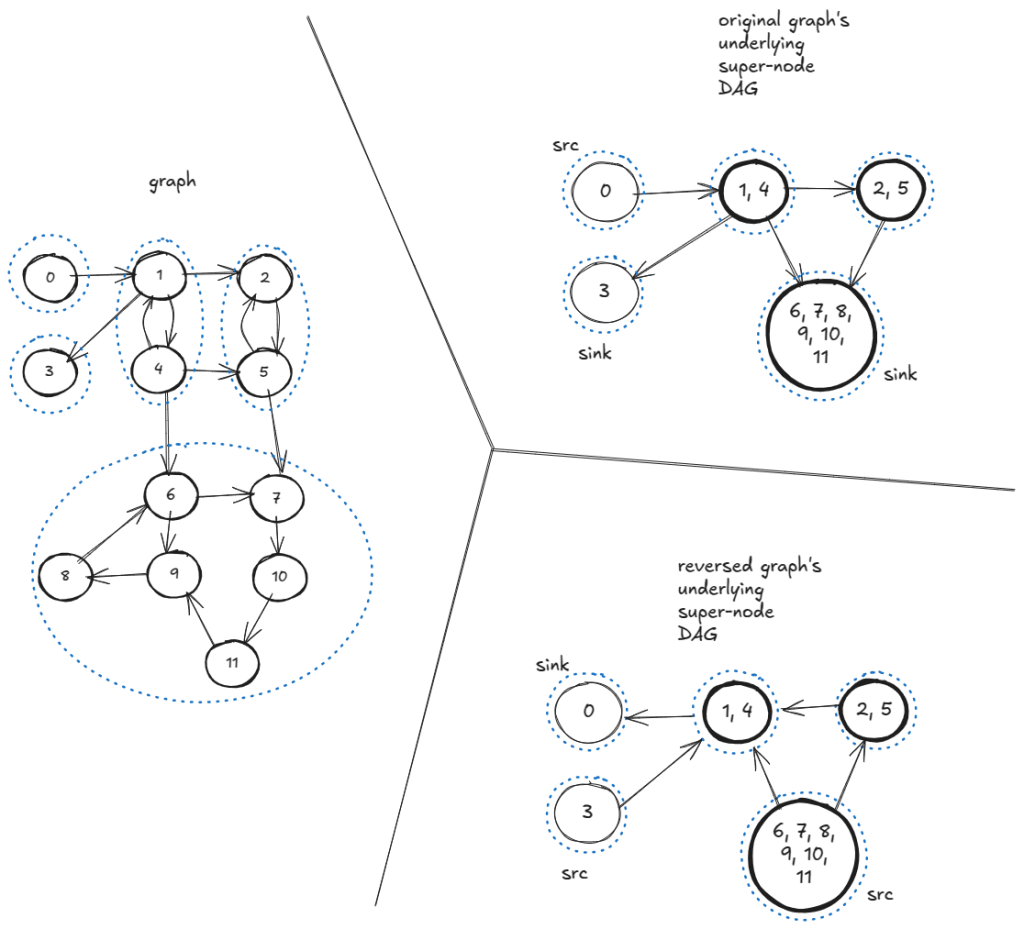
In a strongly connected component, for every vertex-pair: $(u, v)$ , there is a directed path from $u$ to $v$ and a directed path from $v$ to $u$ . There are five strongly connected components in the below directed graph.

Strongly connect component $V_s = \bigcup_{u \in V, v \in V}\left\{ u, v \ : \ \texttt{haspath}(u, v) \wedge \texttt{ haspath}(v, u) \right\}$ . Note, $V_s$ is an equivalence class for the relation $\texttt{haspath}(\cdot)$ . As a result, strongly connected components partition the graph.

For every strongly connected component, if we collapse all vertices within that component into one super-node, we get a DAG of super-nodes.

Insight: In the super-node DAG, if we run DFS within a “sink” super node, the DFS will never leave that super-node or strongly connected component.

Therefore, to find strongly connected components, we can run the undirected graph connected component finding DFS here for the directed graph, but we have to process the vertices in the order of “sink” towards “src”.

The vertex having the highest DFS post time is a “src”. So, to find the “sink”, we can run DFS on the reversed graph and take the highest post in that one. In other words, running undirected connected component (cc) DFS in the decreasing post order of the reversed graph is same as running cc DFS from sink to src of the original graph.

Time and space: $\mathcal{O}( |V| + |E| )$ .

from collections import defaultdict
from typing import Dict, List

def cc_explore(u, adj_list, visited, tic, cc) -> None:
    visited[u] = True
    cc[u] = tic
    for v in adj_list[u]:
        if visited[v]:
            continue
        cc_explore(v, adj_list, visited, tic, cc)

def cc_dfs(adj_list, sorted_nodes) -> List[int]:
    n = len(sorted_nodes)
    visited = [False] * n
    cc = [0] * n
    tic = 1
    for u in sorted_nodes:
        if visited[u]:
            continue
        cc_explore(u, adj_list, visited, tic, cc)
        tic += 1
    return cc

def explore_post(u, adj_list, visited, post_order) -> None:
    visited[u] = True
    
    for v in adj_list[u]:
        if visited[v]:
            continue
        explore_post(v, adj_list, visited, post_order)
    
    post_order.append(u)

def decreasing_post_order(adj_list) -> List[int]:
    n = len(adj_list)
    visited = [False] * n
    post_order = []
    for u in range(n):
        if visited[u]:
            continue
        explore_post(u, adj_list, visited, post_order)
    return post_order[::-1]

def reverse_adj_list(adj_list: List[List[int]]) -> List[List[int]]:
    n = len(adj_list)
    rev_list = [[] for _ in range(n)]
    for u in range(n):
        for v in adj_list[u]:
            rev_list[v].append(u)
    return rev_list

def strongly_connected_components(adj_list: List[List[int]]) -> Dict[int, List[int]]:
    rev_adj_list = reverse_adj_list(adj_list)
    sink_to_src = decreasing_post_order(rev_adj_list)
    cc = cc_dfs( adj_list, sink_to_src )
    cc_map = defaultdict(list)
    for u, comp in enumerate(cc):
        cc_map[comp].append(u)
    return cc_map

adj_list_strong_cc = [
    [1], # 0
    [2, 3, 4], # 1
    [5], # 2
    [], # 3
    [1, 5, 6], # 4
    [2, 7], # 5
    [7, 9], # 6
    [10], # 7
    [6], # 8
    [8], # 9
    [11], # 10
    [9]  # 11
]

strong_cc = strongly_connected_components( adj_list_strong_cc )
print(f"{strong_cc=}")

# strong_cc=defaultdict(<class 'list'>, {5: [0], 4: [1, 4], 3: [2, 5], 2: [3], 1: [6, 7, 8, 9, 10, 11]})

BFS

We visit the not-visited nodes in a layer-by-layer manner. All adjacent to‘s first, then adjacent-adjacent to‘s etc.

def explore(src, adj_list, visited, tree):
    visited.add(src)
    tree.append(src)
    q = deque([src])
    while q:
        u = q.popleft()
        for v in adj_list[u]:
            if v in visited:
                continue
            visited.add(v)
            tree.append(v)
            q.append(v)

def bfs(adj_list) -> List[List[str]]:
    visited = set()
    forest = []
    for u in adj_list:
        if u in visited:
            continue
        tree = []
        explore(u, adj_list, visited, tree)
        forest.append(tree)
    return forest

adj_list = {
    "A": ["B", "E"],
    "B": ["A"],
    "C": ["D", "G", "H"],
    "D": ["C", "H"],
    "E": ["A", "I", "J"],
    "F": [],
    "G": ["C", "H", "K"],
    "H": ["C", "D", "G", "K", "L"],
    "I": ["E", "J"],
    "J": ["E", "I"],
    "K": ["G", "H"],
    "L": ["H"]
}

forest = bfs(adj_list)
print(f"{forest=}")

# forest=[['A', 'B', 'E', 'I', 'J'], ['C', 'D', 'G', 'H', 'K', 'L'], ['F']]

Shortest undirected, unweighted path distances from a source

Time: $\mathcal{O}( |V| + |E| )$ , space: $\mathcal{O}(V)$ .

def shortest_path_distance_bfs(src, adj_list) -> Dict[str, int]:
    dist = {u: float("inf") for u in adj_list}
    dist[src] = 0
    q = deque([src])
    visited = {src}
    while q:
        u = q.popleft()
        for v in adj_list[u]:
            if v in visited:
                continue
            visited.add(v)
            dist[v] = dist[u] + 1
            q.append(v)
    return dist

adj_list = {
    "A": ["B", "S"],
    "B": ["A", "C"],
    "C": ["B", "S"],
    "D": ["E", "S"],
    "E": ["D", "S"],
    "S": ["A", "C", "D", "E"]
}

dist = shortest_path_distance_bfs("S", adj_list)
print(f"{dist=}")
# dist={'A': 1, 'B': 2, 'C': 1, 'D': 1, 'E': 1, 'S': 0}

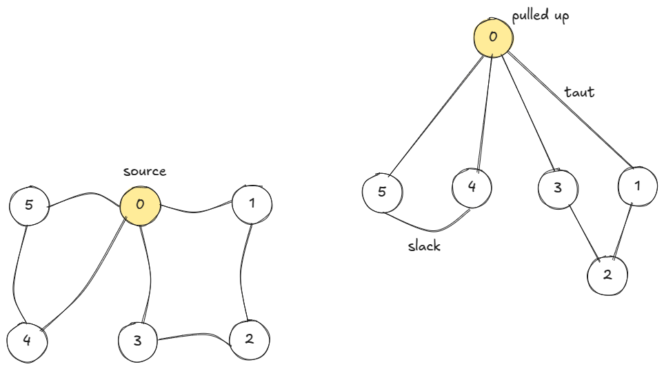
If we think of vertices as balls and edges as strings, BFS is like exploring the taut strings when the source-ball is pulled up.

We can also think BFS as wavefront moving radially outwards from the source one unit distance in one unit time.

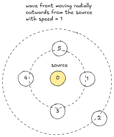
On each iteration, we can process all nodes on the wavefront concurrently.

def shortest_path_distance_bfs_wavefront(src, adj_list) -> Dict[str, int]:
    dist = {u: float("inf") for u in adj_list}
    dist[src] = 0
    q = deque([src])
    visited = {src}
    while q:
        wavefront_len = len(q)
        for _ in range(wavefront_len):
            u = q.popleft()
            for v in adj_list[u]:
                if v in visited:
                    continue
                dist[v] = dist[u] + 1
                visited.add(v)
                q.append(v)
    return dist

Shortest path distances from source with non-negative edge weight

We can extend BFS to accommodate non-negative edge weight (or length) in the following way:

Step 1

Replace an edge $e$ having weight $w > 1$ with $w$ copies of 1-weight edges by inserting $w-1$ virtual nodes. All edges of this new graph has edge length = 1, so we can use BFS.

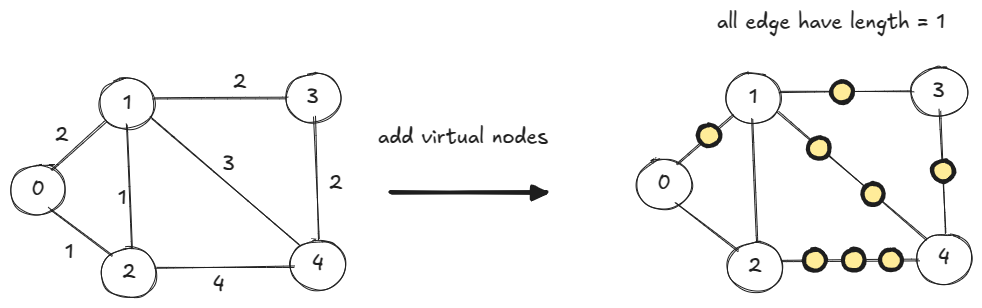
It can be very inefficient. For the below graph, BFS will spend about 100 iterations processing virtual nodes before it finds $\textcircled{1}$ . Then it spends another 50 iterations (via original edge $1 \rightarrow 2$ ) to find $\textcircled{2}$ .

Step 2

We just need to reach $\textcircled{1}$ in one iteration.

Note that, if we ran BFS on the original graph, without inserting virtual nodes, $\textcircled{1}$ would have been the nearest (from the source) node in the queue. So, while the plain BFS always processes the front of the queue, here we need to process the node in the queue that is nearest to source. We replace the plain queue with a min-priority queue with distance from source as key. This is Dijkstra’s shortest path algorithm.

Our min-priority queue should support efficient key update, because, like $\textcircled{2}$ in the above example, we might find shorter paths through other nodes.

Python‘s heapq does not support efficient update of key. So, we use UpdatableMinHeap, which wraps a balanced binary search tree (SortedSet) and a dict.

Time: Heap length is $|V|$ . There are $|V|$ pushes and $|V|$ pops. For each edge we may get an update, so $|E|$ updates. Overall time, $\mathcal{O}\left(\ \left( |V| + |E| \right) \cdot \lg{ |V| }\ \right)$ .

Space: $\mathcal{O}(|V|)$ .

from sortedcontainers import SortedSet
 
class UpdatableMinHeap:
    def __init__(self):
        self.sset = SortedSet()
        self.map = {}
 
    def push(self, item, priority):
        new_entry = (priority, item)
        self.sset.add(new_entry)
        self.map[item] = new_entry
 
    def pop(self):
        _, item = self.sset.pop(0)
        del self.map[item]
        return item
 
    def update(self, item, priority):
        try:
            old_entry = self.map[item]
            del self.map[item]
            self.sset.remove(old_entry)
        except KeyError:
            raise ValueError(f"No '{item}' to update")
        updated_entry = (priority, item)
        self.push(item, priority)
 
    def __bool__(self):
        return bool(self.sset)

def shortest_path_distance_dijkstra(src, adj_list) -> Dict[str, int]:
    dist = {u: float("inf") for u in adj_list}
    dist[src] = 0
    visited = {src}
    q = UpdatableMinHeap()
    q.push(src, 0)
    while q:
        u = q.pop()
        for v, w in adj_list[u]:
            d_v = dist[u] + w
            if v in visited:
                if d_v < dist[v]:
                    dist[v] = d_v
                    q.update(v, d_v)
                continue

            visited.add(v)
            dist[v] = d_v
            q.push(v, d_v)
                
    return dist

adj_list_weighted = {
    "A": [("B", 4), ("C", 2)],
    "B": [("C", 3), ("D", 2), ("E", 3)],
    "C": [("B", 1), ("D", 4), ("E", 5)],
    "D": [],
    "E": [("D", 1)]
}

dist = shortest_path_distance_dijkstra("A", adj_list_weighted)
print(f"{dist=}")
# dist={'A': 0, 'B': 3, 'C': 2, 'D': 5, 'E': 6}

Dijkstra’s shortest path is almost the same as the plain BFS shortest path, except three differences:

Weight: Not always 1.
Queue: Priority queue vs. plain queue
Update: Even if a vertex has been visited, in Dijkstra, if we find a better distance, we allow update.

The assumption of non-negative edge weight is used during update. We update $v$ without checking if it is in the heap:

                if (d_v := dist[u] + w) < dist[v]:
                    dist[v] = d_v
                    q.update(v, d_v)

With non-negative edge weights, $dist[u] + w < dist[v]$ can be true only if $u$ is closer to the src than $v$ . As a result, these $u$ ‘s will be popped before $v$ . Once $v$ is popped, no $u$ exists for which $dist[u] + w < dist[v]$ can be true. As a result, we would not be trying to update a non-existent $v$ .

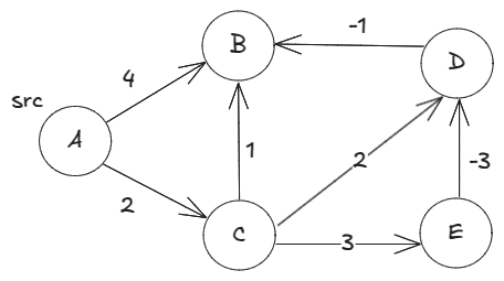
With the below graph with negative edge weights, the update will fail. Because, $\textcircled{B}$ has a better update from $\textcircled{D}$ which is further away from the src. So, when we try to update dist["B"] with dist["D"] + (-4), $\textcircled{B}$ has already been popped and we get ValueError:

adj_list_weighted_neg = {
    "A": [("B", 4), ("C", 2)],
    "B": [],
    "C": [("B", 1), ("D", 3)],
    "D": [("B", -4)]
}

dist = shortest_path_distance_dijkstra("A", adj_list_weighted_neg)
print(f"{dist=}")

# ValueError: No 'B' to update.

Shortest path distances from source with negative edge weight

Looking at Dijkstra’s update, the loop maintains the invariant: dist[v] is either overestimate or exactly correct — it cannot go too low. It cannot go too low because, updates are happening along some neighbor aka along some valid path.

                if (d_v := dist[u] + w) < dist[v]:
                    dist[v] = d_v
                    q.update(v, d_v)

So, updates are actually safe. What if we just relaxed: if $v$ does not exist in the queue, it’s ok, just update dist[v] anyway.

The relaxed Dijkstra works for the below graph with negative weight:

def shortest_path_distance_dijkstra_relaxed(src, adj_list) -> Dict[str, int]:
    dist = {u: float("inf") for u in adj_list}
    dist[src] = 0
    q = UpdatableMinHeap()
    q.push(src, 0)
    visited = {src}
    while q:
        u = q.pop()
        for v, w in adj_list[u]:
            d_v = dist[u] + w
            if v in visited:
                if d_v < dist[v]:
                    try:
                        q.update(v, d_v)
                    except ValueError:
                        pass
                    finally:
                        dist[v] = d_v
                continue
            dist[v] = d_v
            visited.add(v)
            q.push(v, d_v)
    return dist

adj_list_weighted_neg = {
    "A": [("B", 4), ("C", 2)],
    "B": [],
    "C": [("B", 1), ("D", 3)],
    "D": [("B", -4)]
}

dist = shortest_path_distance_dijkstra_relaxed("A", adj_list_weighted_neg)
print(f"{dist=}")
# dist={'A': 0, 'B': 1, 'C': 2, 'D': 5}

However, even the relaxed Dijkstra cannot correctly find the shortest distances for the below graph with negative edge weights:

$\textcircled{B}$ has a shortest path distance of 1 via $\textcircled{E}$ and $\textcircled{D}$ , but the relaxed Dijkstra gives dist["B"] = 3.

adj_list_weighted_neg2 = {
    "A": [("B", 4), ("C", 2)],
    "B": [],
    "C": [("D", 2), ("E", 3)],
    "D": [("B", -1)],
    "E": [("D", -3)]
}
dist = shortest_path_distance_dijkstra_relaxed("A", adj_list_weighted_neg2)
print(f"{dist=}")
# dist={'A': 0, 'B': 3, 'C': 2, 'D': 2, 'E': 5}

The issue is: since $\textcircled{E}$ is furthest from the src, it is processed in the last iteration. As a result, it barely had time to update dist["D"] along the edge $\textcircled{E} \rightarrow \textcircled{D}$ and misses updating dist["B"] along the edge $\textcircled{D} \rightarrow \textcircled{B}$ .

Letting enough updates happen will ensure all distances have settled to their minimum values. The longest shortest path in a $|V|$ vertex graph has $(|V|-1)$ edges. So, we shall let each edge be updated $(|V|-1)$ times. This is Bellman-Ford algorithm.

Time: $\mathcal{O}(|V| \cdot |E|)$ .

def shortest_path_distance_bellman_ford(src, adj_list) -> Dict[str, int]:
    dist = {u: float("inf") for u in adj_list}
    dist[src] = 0
    vertex_count = len(adj_list)
    for _ in range(vertex_count-1):
        for u in adj_list:
            for v, w in adj_list[u]:
                dist[v] = min(dist[v], dist[u]+w)
    return dist

adj_list_weighted_neg2 = {
    "A": [("B", 4), ("C", 2)],
    "B": [],
    "C": [("D", 2), ("E", 3)],
    "D": [("B", -1)],
    "E": [("D", -3)]
}
dist = shortest_path_distance_bellman_ford("A", adj_list_weighted_neg2)
print(f"{dist=}")
# dist={'A': 0, 'B': 1, 'C': 2, 'D': 2, 'E': 5}

Note, the shortest path distance question is ill-posed for a graph with a negative cycle — a cycle whose edge-weights sum up to a negative number. Because, we can always find a shorter path by circling along the negative cycle. If we let all edges be updated $|V|$ time instead of Bellman-Ford’s $(|V|-1)$ times, then in the last iteration an update will still occur if and only if the graph has a negative cycle. We can use this fact to piggy-back on the distance finding to detect the presence of a negative cycle.

Shortest path distance for Directed Acyclic Graph (DAG)

A DAG does not have a cycle, so it cannot have negative cycles. Shortest path distance question is never ill-posed for DAGs. Additionally, if we process the edges in the topological order (say left-to-right) of vertices, the edges will always flow rightwards. As a result, we can perform a single update (instead of $(|V|-1)$ ) of the edges in topological order and be done.

Time: $\mathcal{O}(|V| + |E|)$ .

def sorted_topologically(adj_list) -> List[str]:
    ind = {u: 0 for u in adj_list}
    for u in adj_list:
        for v, _ in adj_list[u]:
            ind[v] += 1
    sources = [u for u, d in ind.items() if d == 0]
    topo = []
    while sources:
        topo.extend(sources)
        new_sources = []
        for u in sources:
            for v, _ in adj_list[u]:
                ind[v] -= 1
                if ind[v] == 0:
                    new_sources.append(v)
        sources = new_sources
    return topo

def shortest_path_distance_dag(src, adj_list) -> Dict[str, int]:
    dist = {u: float("inf") for u in adj_list}
    dist[src] = 0
    for u in sorted_topologically(adj_list):
        for v, w in adj_list[u]:
            dist[v] = min(dist[v], dist[u]+w)
    return dist

In fact, the below graph where relaxed Dijkstra failed and we used Bellman-Ford, is actually a DAG. So, instead of Bellman-Ford’s quadratic time, we could get away with linear time.

adj_list_weighted_neg2 = {
    "A": [("B", 4), ("C", 2)],
    "B": [],
    "C": [("D", 2), ("E", 3)],
    "D": [("B", -1)],
    "E": [("D", -3)]not reachable from src
}
dist = shortest_path_distance_dag("A", adj_list_weighted_neg2)
print(f"{dist=}")
# dist={'A': 0, 'B': 1, 'C': 2, 'D': 2, 'E': 5}

unreasonably effective

Graph Traversal

DFS

Is undirected graph connected?

Categorize directed edges

Is directed graph acyclic?

Topological sort

By DFS post

By in-degree

All topological orderings

All directed cycles

Strongly connected components of directed graph

BFS

Shortest undirected, unweighted path distances from a source

Shortest path distances from source with non-negative edge weight

Step 1

Step 2

Shortest path distances from source with negative edge weight

Shortest path distance for Directed Acyclic Graph (DAG)

Leave a comment Cancel reply

Graph Traversal

DFS

Is undirected graph connected?

Categorize directed edges

Is directed graph acyclic?

Topological sort

By DFS post

By in-degree

All topological orderings

All directed cycles

Strongly connected components of directed graph

BFS

Shortest undirected, unweighted path distances from a source

Shortest path distances from source with non-negative edge weight

Step 1

Step 2

Shortest path distances from source with negative edge weight

Shortest path distance for Directed Acyclic Graph (DAG)

Share this:

Leave a comment Cancel reply